An alternative tool for making plots of various models is to use the sjPlot package. Below are some examples of how to use sjPlot to visualize mixed-effects models fitted with lme4.
We next look at some of the characteristics of these models and data, using sjPlot. We load the library:
library(sjPlot)
Now off we go!
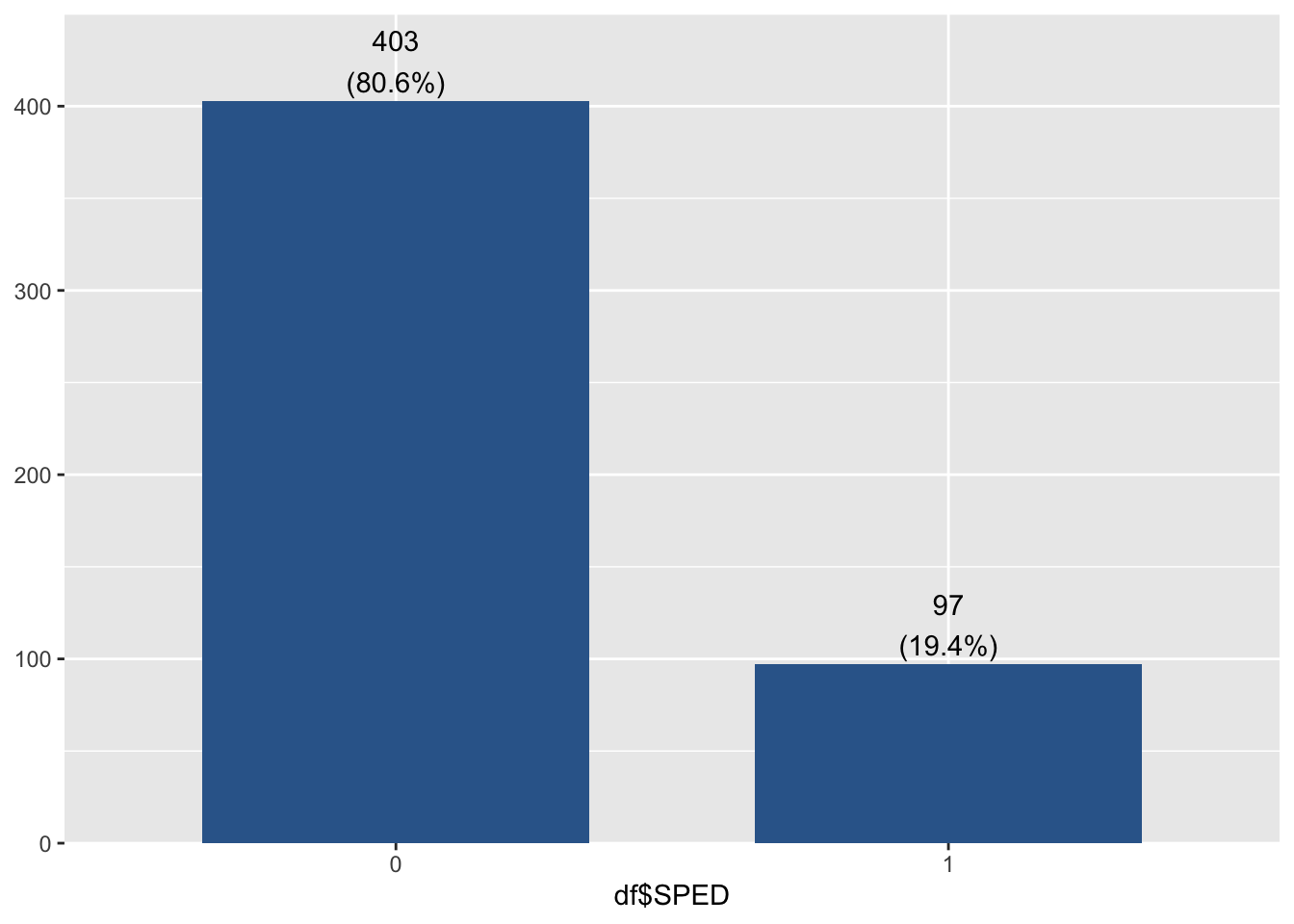
17.1 Frequency Plot for Binary Variable
plot_frq(df$SPED)
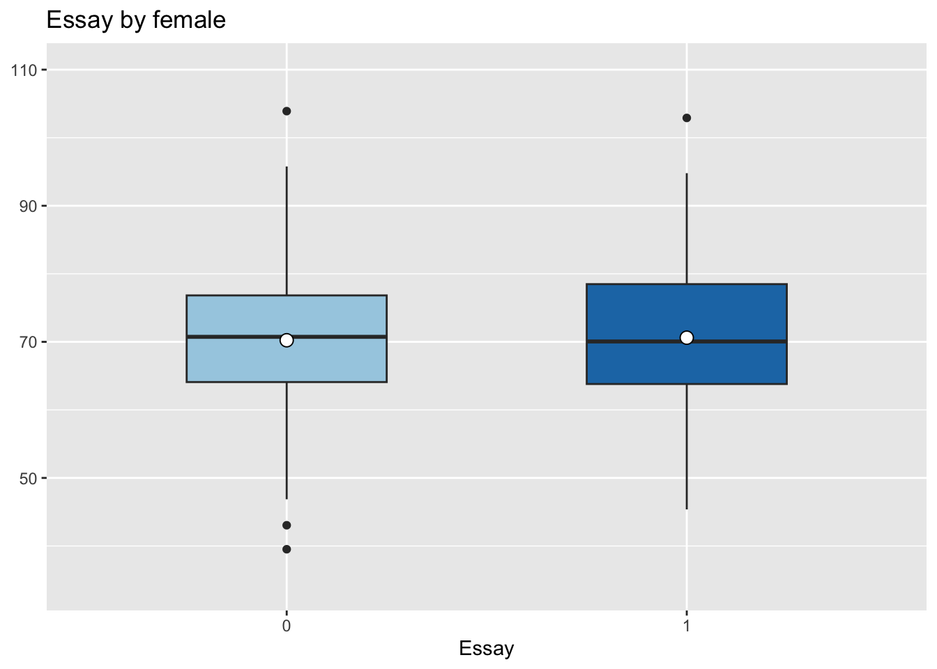
17.2 Boxplot by Group
sjPlot has some general data viz stuff:
plot_grpfrq(var.cnt = df$Essay, var.grp = df$female, type ="box")
Ignoring unknown labels:
• colour : "female"
Warning in rq.fit.br(wx, wy, tau = tau, ...): Solution may be nonunique
Warning in rq.fit.br(wx, wy, tau = tau, ...): Solution may be nonunique
Warning in rq.fit.br(wx, wy, tau = tau, ...): Solution may be nonunique
Warning in rq.fit.br(wx, wy, tau = tau, ...): Solution may be nonunique
Warning in rq.fit.br(wx, wy, tau = tau, ...): Solution may be nonunique
Warning in rq.fit.br(wx, wy, tau = tau, ...): Solution may be nonunique
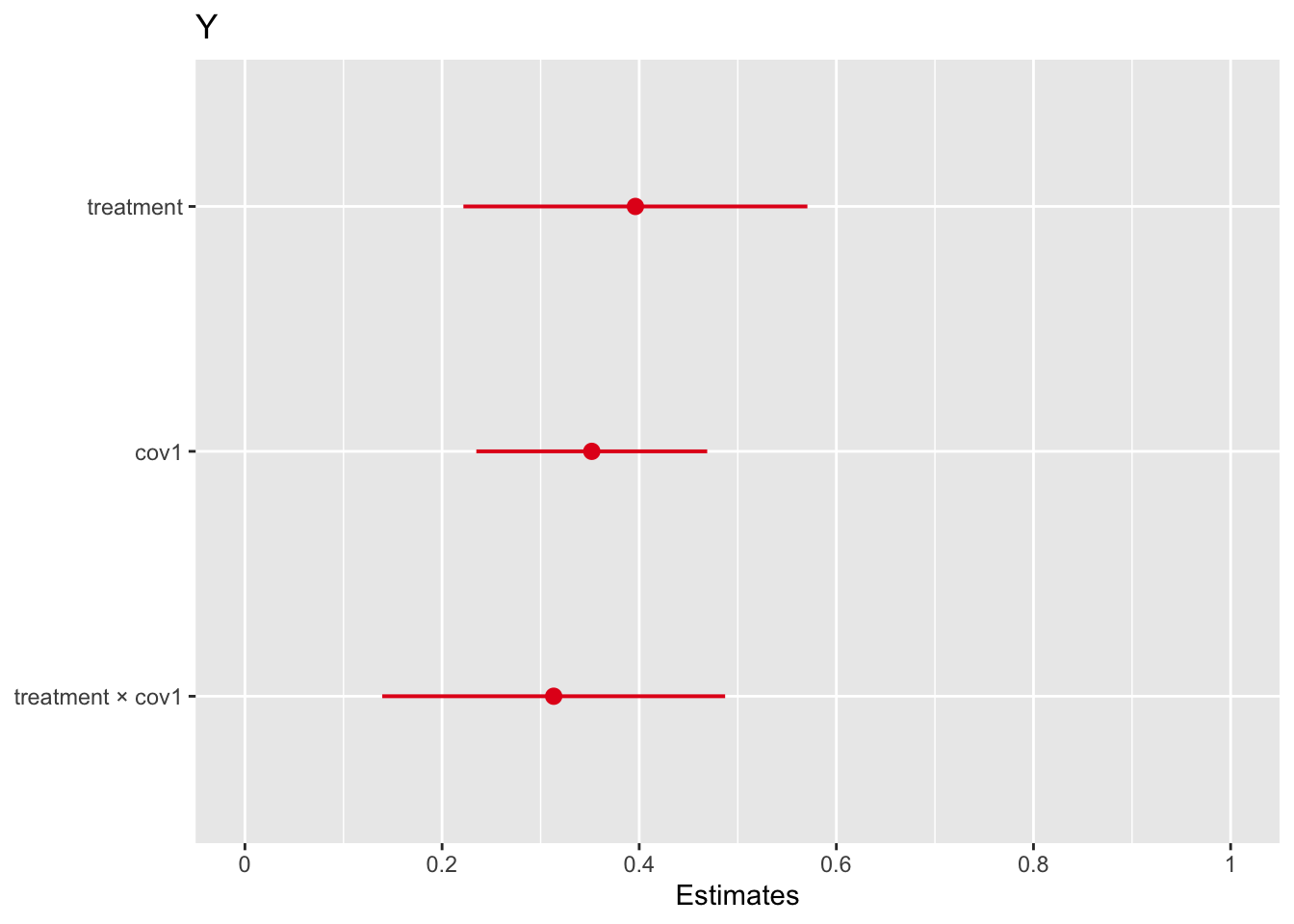
17.3 Fixed Effects Plot
Coefficent plots (see prior chapter):
plot_model(m3, type ="est")
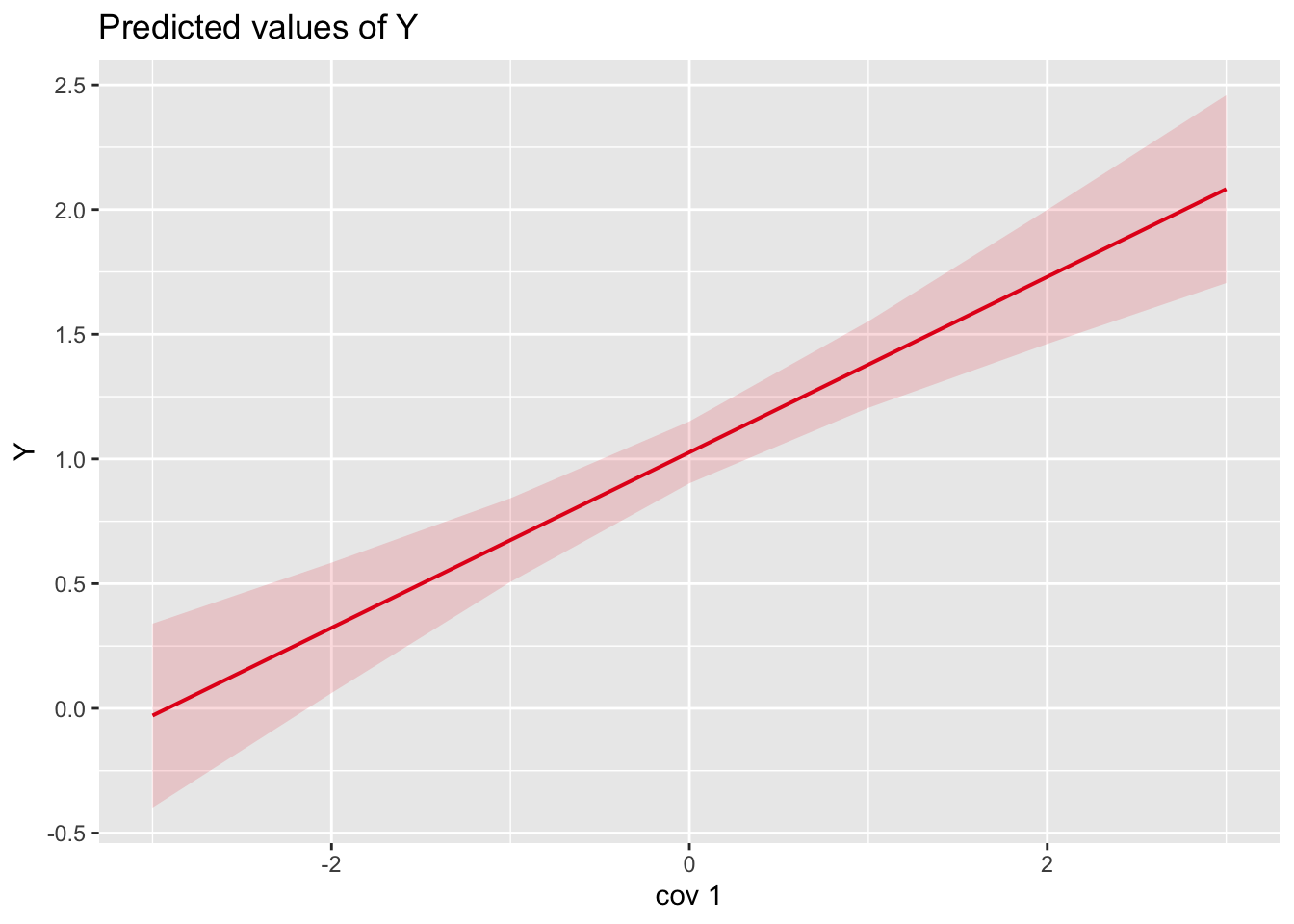
17.4 Marginal Effects (Main Effects)
plot_model(m2, type ="eff", terms =c("cov1", "treatment"))
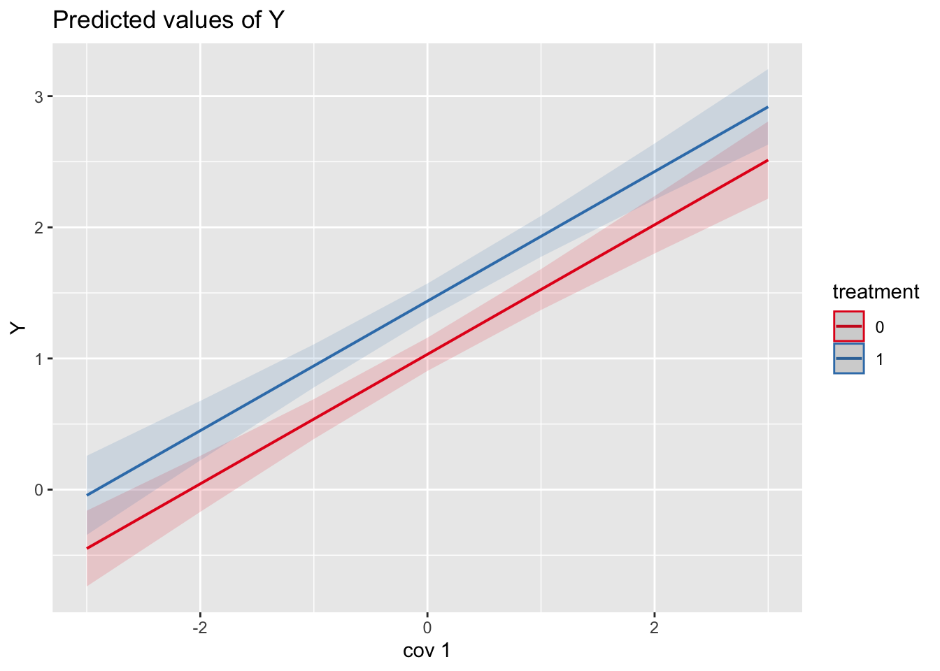
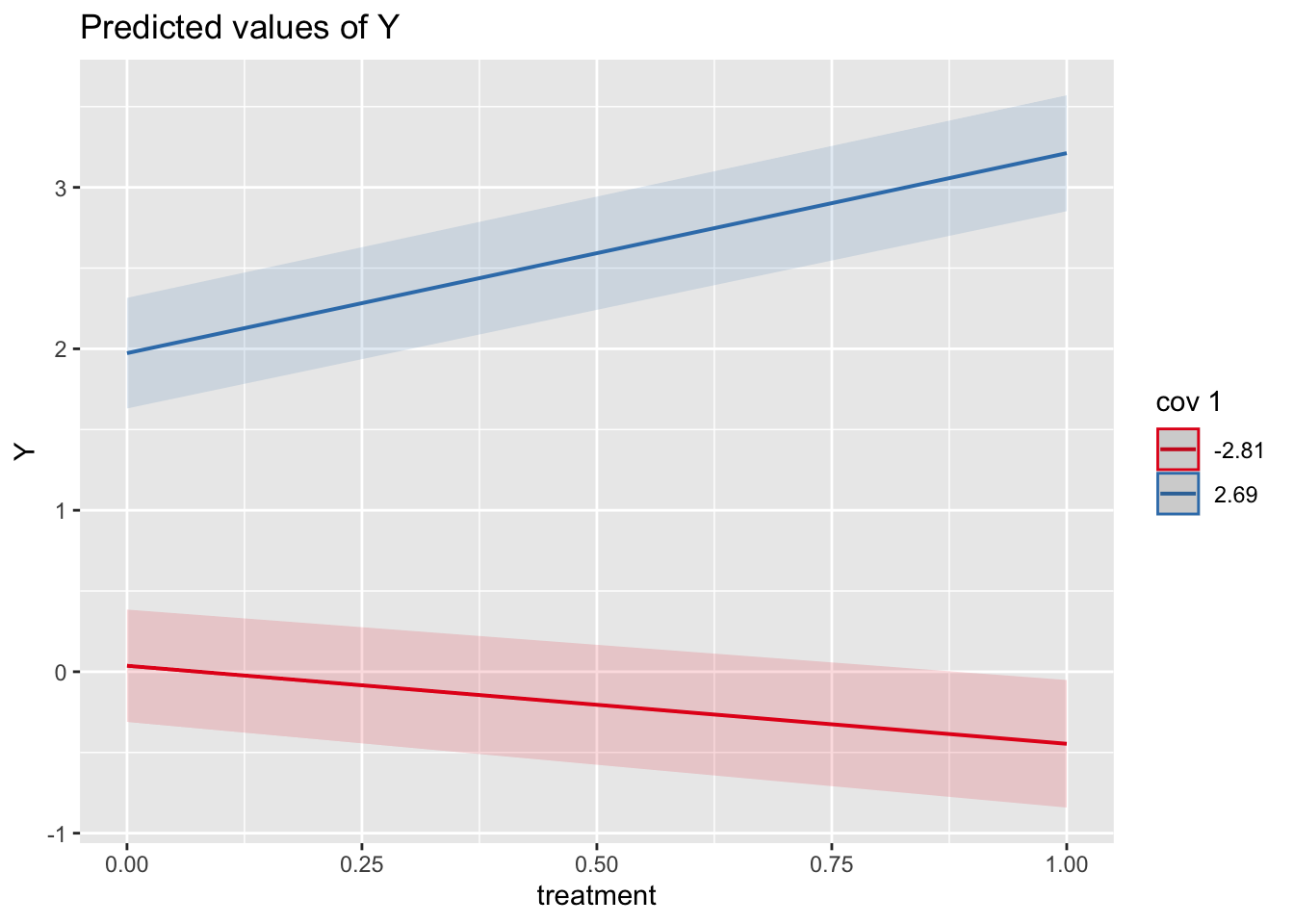
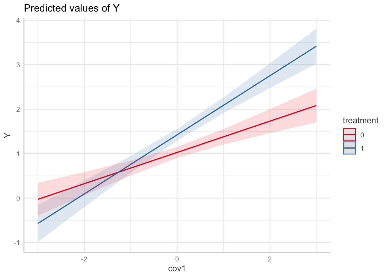
17.5 Interaction Effects Plot
plot_model(m3, type ="int", terms =c("cov1", "treatment"))
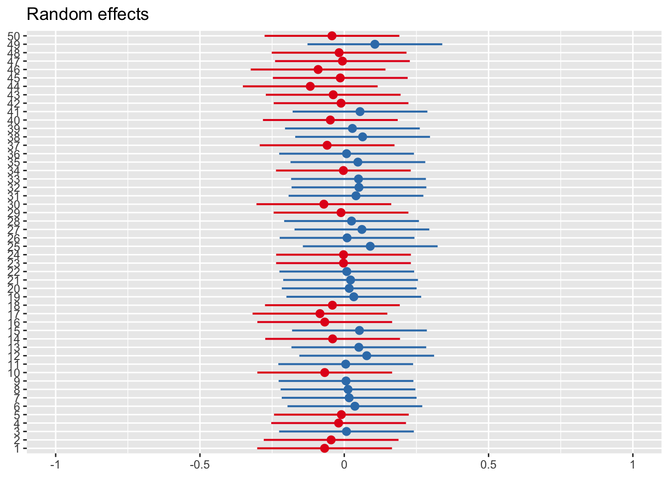
17.6 Random Slopes Plot
plot_model(m3, type ="re", sort.est =TRUE)
Sorting each group of random effects ('sort.all') is not possible when 'facets = TRUE'.
Warning: Using `size` aesthetic for lines was deprecated in ggplot2 3.4.0.
ℹ Please use `linewidth` instead.
ℹ The deprecated feature was likely used in the sjPlot package.
  Please report the issue at <https://github.com/strengejacke/sjPlot/issues>.