24 MLM Assumptions

Author

Luke Miratrix

24.1 Oh, assumptions

There are generally two kinds of assumptions we should worry about the most: ommitted variable bias, and independence assumptions. The latter of these is one we should always think about.

Do read Chapter 9 of R&B, paying attention to their examples and not so much to the mathematical formalism. It has some dense prose, but then moves to specific diagnostics that make what they are talking about much more clear (and it also provides things you can do to check assumptions). The MLM in Plain Language text has some simpler explanations. Also see below for some further notes.

24.2 Ommitted variable bias

Consider the following numerical example:

N = 100
dat = data.frame( X1 = rnorm( N ) )
dat = mutate( dat, 
              X2 = X1 + rnorm( N ),
              Y = 3 + 0.5 * X1 + 1.5 * X2 + rnorm( N ) )

The above makes an X2 that is correlated with X1, and a Y that is a function of both. The true model here is \[ Y_i = \beta_0 + \beta_1 X_{1i} + \beta_2 X_{2i} + \epsilon_{i} \] with coefficents \(\beta = (3, 0.5, 1.5)\).

We fit two models, one with both covariates, and one with only one:

M0 = lm( Y ~ 1 + X1 + X2 , data = dat )
M1 = lm( Y ~ 1 + X1, data = dat )

Our results:

tab_model(M0, M1, p.style = "stars",
          show.ci = FALSE, show.se = TRUE)

	Y		Y
Predictors	Estimates	std. Error	Estimates	std. Error
(Intercept)	3.10 ^***	0.11	2.95 ^***	0.18
X1	0.44 ^**	0.15	1.92 ^***	0.16
X2	1.51 ^***	0.11
Observations	100		100
R² / R² adjusted	0.856 / 0.853		0.584 / 0.580
* p<0.05 p<0.01 * p<0.001

Note our coefficient is completely wrong when we omit a correlated variable. This is omitted variable bias, and in terms of our assumptions we are in a circumstance where the true residuals in our model are not centered around 0 for all values of X1, since they include the X2 effect which is correlated with X1. We can see this as follows:

dat = mutate( dat, e = Y - 3 - 0.5 * X1 )
ggplot( dat, aes( X1, e ) ) +
    geom_point() +
    geom_hline( yintercept = 0 )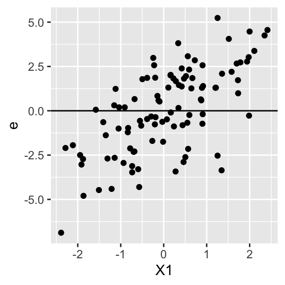

Note how our residuals (which includes X2) are positive for bigger X1, due to the correlation of X1 and X2.

Conclusion: On one hand, we have the wrong estimate for \(\beta_1\). On the other, the estimate we do get is fine if we view it as the best description of the data. We just need to remember that the interpretation of our coefficient includes the confounding effect of X2 on X1.

In this vein:

Q: You mentioned during class that we don’t care too much about assumptions when looking at trends in the data. However, if we are trying to draw causal inferences, do these assumptions become more important?

A: Even with the assumptions causal inference would depend on the model. Modern causal inference has a hard time with this, so you need other strategies such as quasiexperimental design. Hence my focus on descriptive aspects of data analysis.

24.3 Independence assumptions

The independence assumptions are key. When we do not take violations of independence into account, we can be overly confident of our estimates.

Generally with MLM we should think of these assumptions in terms of how we sampled our data. If we sampled our data by sampling a collection of schools, and then individuals within those schools, then we have two levels. We then need to ask two questions:

Were the schools sampled independently?
Were the students sampled independently within the schools?

If yes to both, we have met both our independence assumptions! We have met them even if the students are clustered in classes within their schools. As long as we did not sample using those classes (or other clusters), we are ok as our sample of students will be representative of the school they are in.

One might then ask, more generally, if there is a problem with clustering if it’s not part of the sampling plan? E.g. if you sampled at the school level and surveyed all students, there is still natural clustering in classrooms: is that a problem? What about unobserved clustering like families, neighborhoods, etc. which are not part of sampling, but do exist naturally in populations?

E.g., see this document which says clustered SEs are not necessary (in OLS) unless sampling was conducted at the cluster-level and that econometricians often overuse them.

This is indeed correct. That being said, we might want to make clusters to investigate how things vary across those clusters.

Q: More generally, is there a problem with clustering if it’s not part of the sampling plan? E.g. if you sampled at the school level and surveyed all students, there is still natural clustering in classrooms: is that a problem? What about unobserved clustering like families, neighborhoods, etc. which are not part of sampling, but do exist naturally in populations? Q: I’ll let Luke respond to how this affects the assumptions later on Piazza. My intuition is that we want to cluster/add levels at these different levels if we believe the outcomes or predictors are correlated Q: Thanks. I remember reading this https://blogs.worldbank.org/impactevaluations/when-should-you-cluster-standard-errors-new-wisdom-econometrics-oracle a few years ago, which says clustered SEs are not necessary (in OLS) unless sampling was conducted at the cluster-level and that econometricians often overuse them, but I am wondering to what degree this holds in MLMs.

A: This is correct. That being said, we might want to make clusters to investigate how things vary across those clusters.

24.4 Number of clusters needed?

Ok, this isn’t an assumption per se, but onwards!

Q: Why should you worry if the number of group is small? (referencing the recap slide)

A: With few clusters, estimation is hard just like having a small dataset with OLS. The variance parameters in particular are difficult.

Q: When you say “at least 20” you mean for the number of j’s, right?

A: Yes, number of clusters. Mostly Harmless Econometrics readers might recall a discussion of 42 clusters (8.2.3), which contributes to this debate of the appropriate level of j-units

24.5 Testing assumptions

Q: How do we test these assumptions?

A: Often with plots, like with classic OLS. for example we can pot a histogram of the residuals and see if they are normally distributed.