In Unit 7 we talked about how we can model residuals around an overall population model using different specified structures on the correlation matrices for the students. This handout extends those topics, using the Raudenbush and Bryk Chapter 6 example on National Youth Survey data on deviant attitudes. We’re going to do a few things:
Reproduce the models in the book, showing you how to get them in R, using the commands lme and gls.
Discuss the relationship between lme and gls, and what it actually means when you include a gls-like “correlation” argument when calling lme. To make a long story short: gls is cleaner and more principled from a mathematical point of view, but in practice you will probably prefer hybrid calls using lme.
Give two ways this stuff can actually be useful – heteroskedasticity and AR[1] – and show how to fit realistic models with either and both. We’ll interpret and check significance of parameters as appropriate.
52.1 National Youth Survey running example
Our running example is the data as described in Raudenbush and Bryk, and we follow the discussion on page 190. These data are the first cohort of the National Youth Survey (NYS). This data comes from a survey in which the same students were asked yearly about their acceptance of 9 “deviant”^[Wow, has the way we talk about things changed over the years.] behaviors (such as smoking marijuana, stealing, etc.). The study began in 1976, and followed two cohorts of children, starting at ages 11 and 14 respectively. We will analyze the first 5 years of data.
At each time point, we have measures of:
ATTIT, the attitude towards deviance, with higher numbers implying higher tolerance for deviant behaviors.
EXPO, the “exposure”, based on asking the children how many friends they had who had engaged in each of the behaviors. Both of these numbers have been transformed to a logarithmic scale to reduce skew.
For each student, we also have:
Gender (binary)
Minority status (binary)
Family income, in units of $10K.
One reasonable research question would to describe how the cohort evolved. For this question, the parameters of interest would be the average attitudes at each age. Standard deviations and intrasubject correlations are, as is often but not always the case, simply nuisance parameters. Still, the better we can do at realistically modeling these nuisance parameters, the more precision we will have for the measures of interest, and the power we will have to test relevant hypotheses.
52.1.1 Getting the data ready
We’ll focus on the first cohort, from ages 11-15. First, let’s read the data.
Note that this table is in “wide format”. That is, there is only one row for each student, with all the different observations for that student in different columns of that one row.
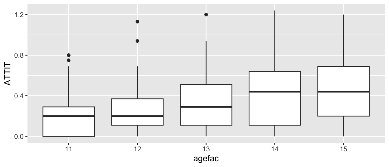
Note some features of the data: First, we see that ATTIT goes up over time. Second, we see the variation of points also goes up over time. This is heteroskedasticity.
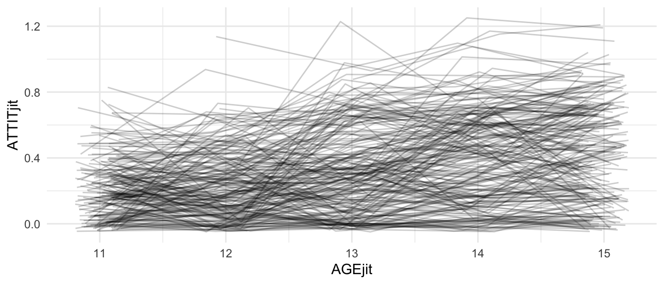
Note how we have correlation of residuals, in that some students are systematically low and some are systematically higher (although there is a lot of bouncing around).
52.2 Representation of error structure
In our data, we have 5 observations \(y_{it}\) for each subject i at 5 fixed times \(t=1\) through \(t=5\). Within each person \(i\) (where person is our Level-2 group, and time is our Level-1), we can write
\[\begin{pmatrix}y_{i1}\\
y_{i2}\\
y_{i3}\\
y_{i4}\\
y_{i5}
\end{pmatrix} = \left(\begin{array}{c}
\mu_{1i}\\
\mu_{2i}\\
\mu_{3i}\\
\mu_{4i}\\
\mu_{5i}
\end{array}\right) + \left(\begin{array}{c}
\epsilon_{1i}\\
\epsilon_{2i}\\
\epsilon_{3i}\\
\epsilon_{4i}\\
\epsilon_{5i}
\end{array}\right)\] where our set of 5 residuals are the random part, distributed as
The key part is the correlation between the residuals at different times. We call our entire covariance matrix \(\Sigma\). This matrix describes how the residuals within a single individual (with 5 time points of observation) are correlated.
Our regression model gives us the mean vector for any given student (e.g., \((\mu_{1i}, \ldots, \mu_{5i})\) would be \(X_i'\beta\), where \(X_i\) is a \(5 \times p\) matrix of covariates for student \(i\), and \(\beta\) is our fixed effect parameter vector. \(X_i\) would have one row per time point and time would be one of the columns, to give our predictions for our 5 time points.
Our error structure model gives us the distribution of the \((\epsilon_{1i}, \ldots, \epsilon_{5i})\) for student \(i\). Different ideas about the data generating process lead to different correlation structures here. We saw a couple of those in class.
52.3 Reproducing R&B’s Chapter 6 examples
The above provides a framework for thinking about grouped data: each group (i.e., student) is a small world with a linear prediction line and a collection of residuals around that line. Under this view, we specify a specific structure on how the residuals relate to each other. (E.g., for classic OLS we would have i.i.d. normally distributed residuals, represented as our \(\Sigma\) being a diagonal matrix with \(\sigma^2\) along the diagonal and 0s everywhere else). In R, once we determine what structure we want, we can fit models based on parameterized correlation matrices using the lme command from the nlme package (You may need to first call install.packages("nlme") to get this package), or the gls package.
Let’s load the nlme package now:
library(nlme)
Recall that all of these models include a linear term on age and an intercept (so two fixed effects and no covariate adjustment).
52.3.1 Compound symmetry (random intercept model)
A “compound symmetry” residual covariance structure (all diagonal elements equal, all off-diagonal elements equal) is actually equivalent to a random intercepts model. Thus, there are 2 ways to get this same model:
Other individuals are the same, if they have the same number of time points, given our model. So in this model, we are saying the residuals of a student have the same distribution as any another student with the same number of time points.
52.3.1.1 Comparing the models
These are two very different ways of specifying the same thing, and the parameter estimates we get out are also not the same. Compare the two summary printouts:
summary(modelRE)
Linear mixed-effects model fit by REML
  Data: nys1
        AIC       BIC   logLik
  -204.9696 -185.0418 106.4848

Random effects:
 Formula: ~1 | ID
        (Intercept)  Residual
StdDev:   0.1846979 0.1798237

Fixed effects:  ATTIT ~ AGE
                 Value  Std.Error  DF   t-value p-value
(Intercept) -0.5099954 0.05358498 839 -9.517505       0
AGE          0.0644387 0.00398784 839 16.158810       0
 Correlation:
    (Intr)
AGE -0.969

Standardized Within-Group Residuals:
        Min          Q1         Med          Q3         Max
-2.90522949 -0.64353962 -0.01388485  0.60377631  3.26938845

Number of Observations: 1079
Number of Groups: 239
and
summary(modelCompSymm)
Generalized least squares fit by REML
  Model: ATTIT ~ AGE
  Data: nys1
        AIC       BIC   logLik
  -204.9696 -185.0418 106.4848

Correlation Structure: Compound symmetry
 Formula: ~AGE | ID
 Parameter estimate(s):
      Rho
0.5133692

Coefficients:
                 Value  Std.Error   t-value p-value
(Intercept) -0.5099954 0.05358498 -9.517505       0
AGE          0.0644387 0.00398784 16.158810       0

 Correlation:
    (Intr)
AGE -0.969

Standardized residuals:
        Min          Q1         Med          Q3         Max
-1.77123071 -0.77132300 -0.06434029  0.71151900  3.38387884

Residual standard error: 0.2577787
Degrees of freedom: 1079 total; 1077 residual
These do not look very similar, do they? But wait:
logLik(modelCompSymm)
'log Lik.' 106.4848 (df=4)
logLik(modelRE)
'log Lik.' 106.4848 (df=4)
logLik(modelRE.lme4)
'log Lik.' 106.4848 (df=4)
AIC( modelCompSymm )
[1] -204.9696
AIC( modelRE )
[1] -204.9696
AIC( modelRE.lme4 )
[1] -204.9696
In fact, they have the same AIC, etc., because they are equivalent models.
The lesson is that it’s actually quite hard to see the correspondence between a familiar random-effects model and an equivalent model expressed in terms of a covariance matrix. Sure, we could do a bunch of math and see that in the end they are the same; but that math is already daunting here, and this is the simplest possible situation. The fitted parameters of a covariance-based model are just really hard to interpret in familiar terms.
52.3.2 Autoregressive error structure (AR[1])
One typical structure used for longitudinal data is the “autoregressive” structure. The idea is threefold:
\(Var(u_{it}) = \sigma^2\) - that is, overall marginal variance is staying constant.
\(Cor(u_{it},u_{i(t-1)}) = \rho\) - that is, residuals are a little bit “sticky” over time so residuals from nearby time points tend to be similar.
\(E(u_{it}|u_{i(t-1)},u_{i(t-2)}) = E(u_{it}|u_{i(t-1)})\) - that is, the only way the two-periods-ago measurement tells you anything about the current one is through the intermediate one, with no longer-term effects or “momentum”.
In this case, the unconditional two-step correlation \(Cor(u_{it},u_{i(t-2)})\) is also easy to calculate. Intuitively, we can say that a portion \(\rho\) of the residual “is the same” after each step, so that after two steps the portion that “is the same” is \(\rho\) of \(\rho\), or \(\rho^2\). Clearly, then, after three steps the correlation will be \(\rho^3\), and so on. In other words, the part that “is the same” is decaying in an exponential pattern. Indeed, one could show that (3.), above, requires the correlated part to decay in a memoryless pattern, leaving the Exponential and Hypergeometric distributions (which both show exponential decay) among the few options.
Thus, the within-subject correlation structure implied by these postulates is:
As you can see, this structure takes advantage of the temporal nature of the data sequence to parameterize the covariance matrix with only two underlying parameters: \(\sigma\) and \(\rho\). By contrast, a random intercept model needs the overall \(\sigma\) and variance of intercepts \(\tau\)—also two parameters! Same complexity, different structure.
52.3.2.1 Fitting the AR[1] covariance structure
To get a true AR[1] residual covariance structure, we need to leave the world of hierarchical models, and thus use the command gls. This is just what we’ve discussed in class. However, later on in this document, we’ll see how to add AR[1] structure on top of a hierarchical model, which is messier from a theoretical point of view, but often more useful and interpretable in practice.
Generalized least squares fit by REML
  Model: ATTIT ~ AGE
  Data: nys1
        AIC       BIC   logLik
  -250.4103 -230.4826 129.2051

Correlation Structure: ARMA(1,0)
 Formula: ~AGE | ID
 Parameter estimate(s):
     Phi1
0.6159857

Coefficients:
                 Value  Std.Error   t-value p-value
(Intercept) -0.4534647 0.07515703 -6.033564       0
AGE          0.0601205 0.00569797 10.551218       0

 Correlation:
    (Intr)
AGE -0.987

Standardized residuals:
        Min          Q1         Med          Q3         Max
-1.75013168 -0.81139621 -0.03256558  0.74814629  3.40350724

Residual standard error: 0.2561765
Degrees of freedom: 1079 total; 1077 residual
You have to dig around in the large amount of output to find the parameter estimates, but they are there. Phi1 is the auto-correlation parameter. And the covariance of residuals:
Note that the AIC of our AR[1] model is lower by about 45 than the random intercept model; clearly far superior because it is getting nearby residuals being more correlated, while the random intercept model does not do this. Also see the banding structure of the residual correlation matrix.
52.3.3 Random slopes
In theory, a random slopes model could be done with gls as well as with lme by building the final residual matrices as a function of the random slope parameters; in practice, it’s much more practical just to do it as a hierarchical model with lme:
We have separated our fixed and random components with lme(). We first include a formula with only fixed effects, and then give a right-side-only formula with terms similar to what you’d put in parentheses with lmer() for the random effects.
Our results:
summary(modelRS)
Linear mixed-effects model fit by REML
  Data: nys1
       AIC       BIC   logLik
  -310.125 -280.2334 161.0625

Random effects:
 Formula: ~AGE | ID
 Structure: General positive-definite, Log-Cholesky parametrization
            StdDev     Corr
(Intercept) 0.51024132 (Intr)
AGE         0.05038613 -0.98
Residual    0.16265428

Fixed effects:  ATTIT ~ 1 + AGE
                 Value  Std.Error  DF  t-value p-value
(Intercept) -0.5133250 0.05834087 839 -8.79872       0
AGE          0.0646849 0.00492904 839 13.12323       0
 Correlation:
    (Intr)
AGE -0.981

Standardized Within-Group Residuals:
        Min          Q1         Med          Q3         Max
-2.87852421 -0.55971197 -0.07521191  0.57495076  3.45648135

Number of Observations: 1079
Number of Groups: 239
The first thing to note is the residual covariance matrix comes from the structure of the random intercept and random slope. If you squint hard enough at it, you can begin to see the linear structures in its diagonal and off-diagonal elements. If you graphed it, those structures would jump out more clearly. But in practice, it’s much easier to think of things in terms of the hierarchical model, not in terms of linear structures in a covariance matrix.
Note also that the AIC has dropped by another 60 points or so; we’re continuing to improve the model.
Also note that this is just using a different package to fit the exact same model we would fit using lmer; so far we haven’t taken advantage of the lme command’s additional flexibility.
52.3.4 Random slopes with heteroskedasticity
Relaxing the homoskedasticity assumption in the random slopes model leaves us a bit in between worlds. We’re not fully into the world of GLS, because there are still random effects; but we’re not fully in the world of hierarchical models because there is structure in the residuals within groups. We’ll talk more about this compromise below; for now, let’s just do it.
The key line is the varIdent line: we are saying each age factor level gets its own weight (rescaling) of the residuals—this is heteroskedasticity. In particular, the above says our residual variance will be weighted by a weight for each age factor, so each age level effectively gets its own variance. This is where these models start to get a bit exciting—we have random slopes, and then heteroskedastic residuals (homoskedastic for any given age level), all together. Our fit model:
summary(modelRSH)
Linear mixed-effects model fit by REML
  Data: nys1
        AIC       BIC   logLik
  -312.5801 -262.7608 166.2901

Random effects:
 Formula: ~AGE | ID
 Structure: General positive-definite, Log-Cholesky parametrization
            StdDev     Corr
(Intercept) 0.57693477 (Intr)
AGE         0.05431359 -0.979
Residual    0.14054178

Variance function:
 Structure: Different standard deviations per stratum
 Formula: ~1 | agefac
 Parameter estimates:
       11        12        13        14        15
1.0000000 1.1956077 1.3095863 1.1255204 0.9802346
Fixed effects:  ATTIT ~ AGE
                 Value  Std.Error  DF   t-value p-value
(Intercept) -0.4929012 0.05715886 839 -8.623357       0
AGE          0.0631404 0.00483385 839 13.062128       0
 Correlation:
    (Intr)
AGE -0.981

Standardized Within-Group Residuals:
        Min          Q1         Med          Q3         Max
-2.91635242 -0.54982114 -0.07583457  0.54829526  3.23703249

Number of Observations: 1079
Number of Groups: 239
Note how we have 5 parameter estimates for the residuals, listed under agefac. It appears as if we have more variation in age 13 than other ages. Age 11, the baseline, is 1.0; it is our reference scaling. These numbers are all scaling the overall residual variance parameter \(\sigma^2\) of \(0.1405^2\).
For looking at the covariance structure of the residuals, we use getVarCov() again:
No amount of squinting will show the structure in the original covariance matrix. But when you convert to a correlation matrix, you can again squint and begin to see the linear structures in its diagonal and off-diagonal elements. The same comment as above still applies: in practice, it’s much easier to think of things in terms of the hierarchical model, and only read the diagonals of the covariance matrix.
We can also get our AIC:
summary(modelRSH)$AIC
[1] -312.5801
The AIC has dropped by only another 2.5 points or so; that corresponds to the idea that if one of these two models were exactly true, the odds are about \(e^{2.5/2}\cong 3.5\) in favor of the more complex model. Aside from the fact that that premise is silly – we are pretty sure that neither of these models is the exact truth; and in that case, something like BIC would probably be better than AIC – those odds are also pretty weak; the simpler model is probably better here.
Here’s the reported BICs, by the way: -280.2334145 for the homoskedastic one, and -262.7607678 for the heteroskedastic. As we expected, the simpler model wins that fight. (Though what \(N\) to use for BIC is sometimes not obvious with hierarchical models, so you can’t trust those numbers too much; see the unit on AIC and BIC and model building.)
52.3.5 Fully unrestricted model
OK, let’s go whole hog, and fit the unrestricted model. Again, this means leaving the world of hierarchical models and using gls.
This unrestricted covariance and correlation matrices have the same structures discussed in the book and in class. The AIC has improved by another 6 or 7 points; that’s marginally “significant”, but in practice probably not substantial enough to make up for the massive loss of interpretability. The lesson we should take from that is that there’s not a whole lot of room for improvement just by tinkering with the residual covariance structure; if we want a much better model, we would have to add new fixed or random effects; perhaps other covariates or perhaps a quadratic term in time.
52.4 Having both AR[1] and Random Slopes
Let’s look at an AR1 residual structure along with some covariates in our main model. The following has AR[1] and also a random intercept and slope:
Linear mixed-effects model fit by REML
  Data: nys1
       AIC       BIC   logLik
  -444.203 -389.4427 233.1015

Random effects:
 Formula: ~1 + AGE11 | ID
 Structure: General positive-definite, Log-Cholesky parametrization
            StdDev     Corr
(Intercept) 0.07999781 (Intr)
AGE11       0.03332789 0.718
Residual    0.16897903

Correlation Structure: AR(1)
 Formula: ~1 | ID
 Parameter estimate(s):
      Phi
0.1868886
Fixed effects:  ATTIT ~ AGE11 + EXPO + FEMALE + MINORITY + log(INCOME + 1)
                      Value  Std.Error  DF   t-value p-value
(Intercept)      0.26483469 0.04070122 838  6.506800  0.0000
AGE11            0.04972825 0.00463402 838 10.731129  0.0000
EXPO             0.31452987 0.02489980 838 12.631823  0.0000
FEMALE          -0.01661080 0.02027639 235 -0.819219  0.4135
MINORITY        -0.06296592 0.02676263 235 -2.352755  0.0195
log(INCOME + 1) -0.00943584 0.02359588 235 -0.399893  0.6896
 Correlation:
                (Intr) AGE11  EXPO   FEMALE MINORI
AGE11           -0.123
EXPO            -0.064 -0.225
FEMALE          -0.181 -0.038  0.171
MINORITY        -0.491  0.008  0.011 -0.030
log(INCOME + 1) -0.923 -0.004  0.084 -0.054  0.407

Standardized Within-Group Residuals:
        Min          Q1         Med          Q3         Max
-2.61795250 -0.58685208 -0.08121038  0.57649581  2.82037550

Number of Observations: 1079
Number of Groups: 239
In order to get this model to converge, we had to use the lmeControl command above; without it, the model doesn’t converge due to not reaching a max in the given number of iterations. The lmeControl with optim apparently turns up the juice so it converges without complaint.
Let’s compare our fit model to the same model without AR1 correlation
The AR1 model has a notably lower AIC and thus is significantly better:
anova( model1simple, model1 )
             Model df       AIC       BIC   logLik   Test  L.Ratio p-value
model1simple     1 10 -436.8027 -387.0206 228.4014
model1           2 11 -444.2030 -389.4427 233.1015 1 vs 2 9.400292  0.0022
Autoregression involves only a single extra parameter–the autoregressive correlation coefficient.
Our hybrid model is actually kind of mixed up, conceptually. We allowed a random slope on age, and also an autoregressive component by age. Thus, we effectively allowed the covariance matrix to vary in two different ways, at two different levels of our modeling.
In fact, as we’ve seen in class, any random effects, whether they be on slope or intercept, are actually equivalent to certain ways of varying the variance-covariance matrix of the residuals within each group. For instance, random intercepts are equivalent to compound symmetry. Thus, by including both random intercepts and AR1 correlation in the above model, we’ve effectively fit a model that allows any covariance matrix that can be expressed as a sum of a random slope covariance matrix (with 2 parameters plus a scaling factor) and an AR1 covariance matrix (with 1 parameter plus a scaling factor). That makes 5 degrees of freedom total for our covariance matrix. This is many fewer than the 15 for a fully unconstrained matrix, for comparison.
Conceptually this model is nice: people have linear growth trends, but vary around those growth trends in an autoregressive way.
52.5 The Kitchen sink: building complex models
Which brings us to the next point: how do you actually use this stuff in practice? Ideally, you’d like both the interpretability (and robustness against MAR missingness) of hierarchical models, along with the ability to add additional residual structure such as AR[1] and/or heteroskedastic residuals. The good news is, you can get both. The bad news is, there’s a bit of a potential for bias due to overfitting.
For instance, imagine you use both random effects and AR[1]. Say that for a given subject you have 5 time points, and all of them are above the values you would have predicted based on fixed effects alone. That might be explained by an above-average random effect, or by a set of correlated residuals that all came in high. Whichever one of these is the “true” explanation, the MLE will tend to parcel it out between the two. This can lead to downward bias in variance and/or correlation parameter estimates, especially with small numbers of observations per subject–the variation gets pushed into just assuming the residuals are correlated due to the auto-regressive structure.
Still, as long as your focus is on location parameters such as true means or slopes, having hybrid models can be a good way to proceed. Let’s explore this by first fitting a “kitchen sink” model for this data, in which we use all available covariates; and seeing how adding heteroskedasticity, AR[1] structure, or both changes it (or doesn’t).
What do we want in this “kitchen sink” model? Let’s first fit a very simple random intercept model with fixed effects for gender, minority status, “exposure”, and log(income), to see which of these covariates to focus on. We use the lmerTest package to get some early \(p\)-values for these fixed effects.
Linear mixed model fit by REML. t-tests use Satterthwaite's method [
lmerModLmerTest]
Formula: ATTIT ~ FEMALE + MINORITY + log(INCOME + 1) + EXPO + (1 | ID)
   Data: nys1

REML criterion at convergence: -265.6

Scaled residuals:
    Min      1Q  Median      3Q     Max
-3.1840 -0.5922 -0.0797  0.6043  2.6319

Random effects:
 Groups   Name        Variance Std.Dev.
 ID       (Intercept) 0.01756  0.1325
 Residual             0.03444  0.1856
Number of obs: 1079, groups:  ID, 239

Fixed effects:
                  Estimate Std. Error         df t value Pr(>|t|)
(Intercept)      3.480e-01  4.195e-02  2.301e+02   8.297    9e-15 ***
FEMALE          -1.835e-02  2.094e-02  2.327e+02  -0.876   0.3819
MINORITY        -5.698e-02  2.789e-02  2.279e+02  -2.043   0.0422 *
log(INCOME + 1)  2.102e-03  2.449e-02  2.272e+02   0.086   0.9317
EXPO             4.516e-01  2.492e-02  1.041e+03  18.122   <2e-16 ***
---
Signif. codes:  0 '***' 0.001 '**' 0.01 '*' 0.05 '.' 0.1 ' ' 1
(The correlation=FALSE shortens the printout.)
Apparently, MINORITY and EXPO are the covariates with significant effects; minority status is correlated with a lower tolerance for deviance, while “deviant” friends are of course correlated positively with tolerance of deviance. Let’s build a few hierarchical models including these in various specifications (can you identify what models are what? Some of these models are not necessarily good choices). We first center our age so we have meaningful intercepts.
Note that the estimates for all the effects are essentially unchanged. However, the AIC is almost 40 points better. Also, because the model has done a better job explaining residual variance, the \(p\)-value for the coefficient on MINORITY has dropped from 0.032 to 0.029, as we can see on the summary display below. This is not a large drop, but a noticeable one:
summary( modelKS5 )
Linear mixed-effects model fit by REML
  Data: nys1
        AIC       BIC   logLik
  -433.5943 -398.7338 223.7972

Random effects:
 Formula: ~1 | ID
        (Intercept)  Residual
StdDev:   0.1186009 0.1864592

Correlation Structure: ARMA(1,0)
 Formula: ~AGE | ID
 Parameter estimate(s):
     Phi1
0.3212696
Fixed effects:  ATTIT ~ MINORITY + age13 + EXPO
                 Value   Std.Error  DF   t-value p-value
(Intercept)  0.3408351 0.011858053 838 28.742920   0.000
MINORITY    -0.0570447 0.025968587 237 -2.196683   0.029
age13        0.0473388 0.004523745 838 10.464512   0.000
EXPO         0.3520799 0.024451130 838 14.399330   0.000
 Correlation:
         (Intr) MINORI age13
MINORITY -0.457
age13    -0.013  0.010
EXPO      0.006 -0.001 -0.224

Standardized Within-Group Residuals:
        Min          Q1         Med          Q3         Max
-2.82097989 -0.65136103 -0.08846076  0.61819746  2.77303796

Number of Observations: 1079
Number of Groups: 239
Is any of this drop in the \(p\)-value due to overfitting? Given the size of the change in AIC, it seems doubtful that that’s a significant factor.
Let’s try including heteroskedasticity, without AR[1]: