data("sleepstudy", package = "lme4")

ggplot( sleepstudy, aes( Days, Reaction, group=Subject ) ) +
  facet_wrap( ~ Subject ) +
  geom_smooth( method="lm", se=FALSE, lwd=0.5, alpha=0.5 ) +
geom_line() 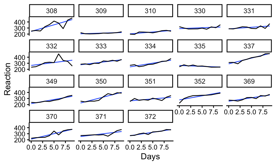
The goal of the ICC is to quantify the proportion of total variance in the outcome that is attributable to between-person differences, relative to within-person differences. With a longitudinal growth model, we are allowing different people to have different baseline levels (the random intercept) and also different growth trajectories (e.g., the random slope, in a linear growth model). To calculate an overall “ICC” we would then want to calculate how much these individual growth trajectories explain.
The easiest way to get a handle on this is to calculate the within and between variation in a bit of a roundabout way: we first calculate total variation of our observations around the overall population growth curve for our estimate of total variation, and then we look at the remaining residual variation beyond the random effects to get within variation. Between variation is then the difference of these quantities.
We next demonstrate on a simple example using the sleepstudy data from the lme4 package. The data look like this:
data("sleepstudy", package = "lme4")
ggplot( sleepstudy, aes( Days, Reaction, group=Subject ) ) +
facet_wrap( ~ Subject ) +
geom_smooth( method="lm", se=FALSE, lwd=0.5, alpha=0.5 ) +
geom_line()
We fit a no-covariate linear growth model to these data. We could fit any other growth model (e.g., quadratic) and everything that follows would be the same.
# Random intercepts for Subject; time (Days) as fixed effect only
m_rs <- lmer(Reaction ~ Days + (1 + Days | Subject), data = sleepstudy,
             REML = TRUE)
arm::display(m_rs)
lmer(formula = Reaction ~ Days + (1 + Days | Subject), data = sleepstudy,
REML = TRUE)
coef.est coef.se
(Intercept) 251.41 6.82
Days 10.47 1.55
Error terms:
Groups Name Std.Dev. Corr
Subject (Intercept) 24.74
Days 5.92 0.07
Residual 25.59
---
number of obs: 180, groups: Subject, 18
AIC = 1755.6, DIC = 1760.3
deviance = 1751.9 Our fit model shows substantial variation in both intercepts and slopes across subjects.
We next calculate our “population level” residuals, and look at the within-person variation around the population curve to get the total variance.
sleepstudy$yhat_pop <- predict(m_rs, re.form = NA)  # population-level predictions

total_var = var( sleepstudy$Reaction - sleepstudy$yhat_pop )
sqrt( total_var )
[1] 47.58125Note the re.form = NA: this means our predict() method predicts from just the fixed effects—our residuals are then distance to the overall population line.
Finally we calculate our ICC as 1 minus the ratio of within-person variance to total variance (which is equivilent to between-person over total, like we normally see, using the idea that total variation is within + between):
1 - sigma(m_rs)^2 / total_var[1] 0.7107124Compare the above ICC to just the random intercept “traditional” ICC:
m_ri <- lmer(Reaction ~ Days + (1 | Subject), data = sleepstudy,
              REML = TRUE)

vc = arm::sigma.hat(m_ri)
vc$sigma$Subject^2 / ( vc$sigma$Subject^2 + vc$sigma$data^2 )
(Intercept)
0.5893089 By including random slopes, we are explaining more of the total variation between people, so the ICC goes up. Arugably our fancy ICC is more authentically breaking down how much is between variation (how are people different) vs. within variation (how are individual observations noise around some fundamental growth trajectory).
We can compare our answers to the performance package’s icc() method:
# Random intercept:
icc(m_ri)
# Intraclass Correlation Coefficient
Adjusted ICC: 0.589
Unadjusted ICC: 0.424# Random slope:
icc(m_rs)# Intraclass Correlation Coefficient
Adjusted ICC: 0.722
Unadjusted ICC: 0.521The “Unadjusted ICC” includes the fixed effects portion of the model (so the overall time trend); it is generally not preferred. But the icc() method seems to have estimated ICCs that make sense!
The ICC in a longitudinal context highlights the stability or consistency of individuals’ scores across measurement occasions around some latent growth trajectory. A high ICC indicates that most of the variability in the outcome lies between individuals, implying the measures will be close to the true curves; a low ICC means outcomes fluctuate more within individuals around their latient growth curves across time points.
We next walk through the steps for building a set of growth models.
Start unconditional. To start building a longitudinal growth model, start with an unconditional model, i.e., don’t include any level-1 or level-2 predictors (other than your time variable). Singer & Willett (2003) call this the “unconditional means model.” This base model will provide useful empirical evidence for determining a proper specification of the individual growth equation and also give you baseline statistics for evaluating more complicated level-2 models.
Calculate ICC. Next calculate ICC as described above to get a sense of whether there is much to explain in terms of between-person variation. If most of the variance is between-persons in the random intercept (level-2), then you’ll use person-level predictors to reduce that variance (i.e., account for inter-person differences). If most of the variance is within-person (level-1 residual variance), you’ll need time-level predictors to reduce that variance (i.e. account for intra-person differences)
You might also tinker with the form of your model at this point, e.g., deciding to move to a quadratic growth model or some other functional form.
Sequentially add predictors. Once you have your baseline model, you can start adding predictors.
Time-invariant predictors always go into the level-2 (subject level) model. Time-varying predictors, by contrast, must appear in the level-1 individual growth model; this is enforced by the time-specific subscript t, which can only appear in level-1.
Time-varying predictors can have information for both level 1 and level 2 (consider that some predictors might generally be high, but vary, for one person and generally be low, but vary, for another person). You can explicitly build a level-2 covariate by group averaging a level 1 covariate, and then build a “pure” level-1 covariate by subtracting the group means from the original predictor. This is group mean centering to achieve a between vs within decomposition, as we have discussed before.
If you are trying to explain growth, you will want to interact your level 2 predictor with the time variable. Just including it without interactions will explain the overall level of outcome only.
Although the order in which you add your predictors predictors (in a series of successive models) may not ultimately matter, general practice is to add level-2 (time-invariant) predictors first.
You could, in principle, have random slopes for some of your time varying (level-1) predictors, allowing their effects to vary across people. Use this approach with caution: if you have only a few measurement points per person, you will not have much ability to estimate many variance components. Generally resist the temptation to automatically allow the effects of time-varying predictors to vary at level-2 unless you have a good reason, and enough data, to do so.
As with all multilevel models, the level of the predictor dictates which variance component it seeks to describe: Level-2 describes level-2 variances and Level-1 describes level-1 variances.
This means, when we include time-invariant (level 2) predictors:
the level-1 variance component, \(\sigma^2_e\), remains pretty stable because time-invariant predictors cannot explain any within-person variation
the level-2 variance components, \(\tau_{00}\) can decrease if the time-invariant predictors explain some of the between-person variation in initial status. If you interact the predictor with time, you could see a reduction in \(\tau_{11}\) if the predictor indeed is able to explain differences in the growth rates.
When we include time-varying predictors:
both level-1 and level-2 variance components might be affected because time-varying predictors can vary both within a person and between people. If you have group-mean centered your level 1 predictor, the level 2 variance should be stable.
we can interpret the resulting decrease in the level-1 variance component as amount of variation in the outcome explained by the time-varying predictors; however, it isn’t meaningful to interpret subsequent changes in level-2 variance components because adding the time-varying predictor changes the meaning of the individual growth parameters, which consequently alters the meaning of the level-2 variances. This means it does not make sense to compare the magnitude of these level-2 variances across successive models.
Level-1 predictors make interpreting longitudinal growth models very, very confusing. You are looking at growth beyond that which is explained by possible changes over time of the level-1 predictors! Use them with care.