35Clarification on Fixed Effects and Identification
Author
Luke Miratrix
This chapter talks a bit more about fixed effects. It starts with an overview of the language used to talk about them, gives a brief bit about underidentification, and then moves to looking at how we can have fixed effects interacted with other covariates. The final parts connect to in-class discussion of fixed effects; in particular it gives a reflection on the four concept questions from Packet 1.2 (the live session slides).
35.1 The language of “Fixed Effects”
People will talk about “fixed effects” in (at least) two ways. The first is when you have a dummy variable for each of your clusters, and you are using OLS regression (not multilevel modeling). In this case you are estimating a parameter for each cluster, and we refer to that collection of estimates and parameters that go with these cluster level dummy variables as “fixed effects” and the model is a “fixed effects model.” The second is when you are using multilevel modeling, such as the following:
When we fit the above model, we will be estimating a grand intercept, and three coefficients for the three variables. Call these \(\beta_0\), \(\beta_1\), \(\beta_2\), and \(\beta_3\). We are also estimating a random intercept and random slope for var1, with each group defined by the id variable having its own random intercept and slope. These are described by a variance-covariance matrix that we have been describing with \(\tau_{00}, \tau_{01}, \tau_{11}\).
Now, the \(\beta\) are the fixed part, or fixed effects, of the model. The \(\tau\) describe the random part or random effects. This is why, in R, we say fixef(M0) to get the \(\beta\). If we say ranef(M0) we get the Empirical Bayes estimates of the random parts for each cluster. If we say coef(M0) R adds all this together to give the sum of the fixed part and random part, for each cluster defined by id.
Read Gelman and Hill 12.3 for more on this sticky language. G&H do not like “fixed effects” as a description because it is so vague.
35.2 Underidentification
If we fit a model with a dummy variable for each cluster, and a level to variable that does not vary within cluster, we say our model is “underidentified.” We say it is underidentified because no matter how much data we have, we will always have an infinite number of parameter values that can describe our model equally well. For example, say our level 2 variable is a dummy variable (e.g., sector). Then a model where we add five to the coefficient of the level 2 variable, and subtract five from all of the fixed effects for the clusters with sector=1 will fit our data just as well as one where we don’t. We can’t tell the difference! Hence we do not have enough to “identify” the parameter values.
35.3 Model syntax: removing the main ses term vs not
Note how when we remove ses via - ses we gain an extra interaction term of ses:id1288. In M1, our ses coefficient is our baseline slope of school 1288. The ses interaction terms are slope changes.
Note how if we add ses to the changes we get back all the slopes in M2:
Bottom line: M1 and M2 are exactly the same in what they are describing, they are just parameterized differently. Anything we learn from one we could learn from the other.
35.3.1 Plot our model
To plot our model we make a dataset of the intercepts and slopes of each school. Doing this with M2 is much easier than M1, since the coefficients are exactly what we want:
lines =data.frame( id =names( coef(M2) )[1:10],inter =coef(M2)[1:10],slope =coef(M2)[11:20] )# we need to fix our IDs. :-(lines$id =gsub( "id", "", lines$id)head( lines )
(The gsub “substitutes” (replaces) the string “id” with “” in all of our ids so we get back to the actual school ids. Otherwise we will not be able to connect these data to our raw students as easily.)
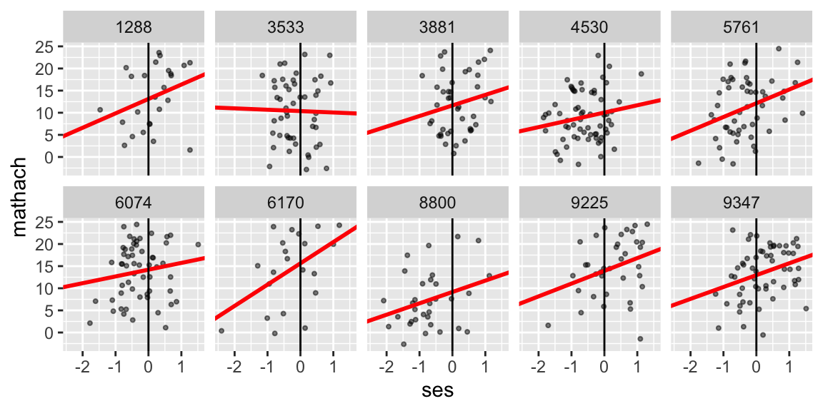
35.3.2 What do the intercepts of any of the lines mean?
The intercepts predict what math achievement a studnet with ses = 0 going to a given school would have. For example, in school 8800, we predict a student with an ses of 0 would have a math achievement of 9.2.
Notice that for some schools the intercept is extrapolating. E.g., most of school 8800’s students are below 0 for ses, and the intercept is thus describing what we expect for students at the higher end of their range. For school 9225, we are seeing a prediction for students a bit below the middle of their range.
35.3.3 What differences, if any, are there between running a new linear model on each school vs. running the interacted model on the set of 10 schools?
The lines would be exactly the same. The standard errors are different. Here is the line on just school 1288:
Call:
lm(formula = mathach ~ 1 + ses, data = s1288)

Residuals:
    Min      1Q  Median      3Q     Max
-15.648  -5.700   1.048   4.420   9.415

Coefficients:
            Estimate Std. Error t value Pr(>|t|)
(Intercept)   13.115      1.387   9.456 2.17e-09 ***
ses            3.255      2.080   1.565    0.131
---
Signif. codes:  0 '***' 0.001 '**' 0.01 '*' 0.05 '.' 0.1 ' ' 1

Residual standard error: 6.819 on 23 degrees of freedom
Multiple R-squared:  0.09628,   Adjusted R-squared:  0.05699
F-statistic:  2.45 on 1 and 23 DF,  p-value: 0.1312
The SEs will be different, however. Compare:
sum =summary( M2 )sum$coefficients[ c(1, 11 ), ]
            Estimate Std. Error   t value     Pr(>|t|)
id1288     13.114937   1.291495 10.154850 9.121968e-22
ses:id1288  3.255449   1.936454  1.681139 9.349559e-02
In this case the SEs are close, but they could be a lot different if we have a lot of heteroskedasticity or the school has few data points so we do a bad job estimating uncertainty.
The key is in the single model we are using all the schools to estimate the residual variance, and this is the number that drives our SE estimates.
35.3.4 Do we trust the red lines on the plot? Why or why not?
We trust them because they are driven just by the school data, so they are essentially unbiased. But these are small datasets, so they are unstable.
35.3.5 What about the variability in the slopes and intercepts of the red lines?
The variation is not to be trusted. The slopes are varying because of measurement error. For example, it is unlikely school 3533 really has a negative slope. It is more likely we just got some low performing high ses kids by happenstance in our sample. Similarly, it is unlikely school 6170 has such a steep slope. It has few kids, and the kid with less than -2 ses and a very low math achievment is likely an influential point in that regression.
Antonakis, John, Nicolas Bastardoz, and Mikko Rönkkö. 2019. “On Ignoring the Random Effects Assumption in Multilevel Models: Review, Critique, and Recommendations.”Organizational Research Methods 24 (2): 443–83. https://doi.org/10.1177/1094428119877457.