23  A visual guide to parameters

In this guide I am going to generate a different collection of datasets for a variety of different null hypothesis so we can see what each hypothesis means.

The main model, in the classic two-level hierarchical linear model form, is as follows:

Level-1 Model (Within-Group): \[ Y_{ij} = \beta_{0j} + \beta_{1j} SES_{ij} + \epsilon_{ij} \] where \(Y_{ij}\) is the outcome and \(SES_{ij}\) is the predictor for individual \(i\) in school \(j\), and \(\epsilon_{ij}\) is the student residual (normally distributed, etc.).

Level-2 Model (Between-Group): \[ \begin{aligned} \beta_{0j} &= \gamma_{00} + \gamma_{01} \text{sector}_{j} + u_{0j} \\ \beta_{1j} &= \gamma_{10} + \gamma_{11} \text{sector}_{j} + u_{1j} \end{aligned} \] where $ _{j} $ is the indicator for Catholic or public for school \(j\), and \(u_{0j}\) and \(u_{1j}\) are the random effects for intercept and slope, respectively, for school \(j\).

The random effects $ (u_{0j}, u_{1j}) $ are assumed to be multivariate normal with a mean of zero and a covariance matrix \(\Sigma\): \[ \begin{pmatrix} u_{0j} \\ u_{1j} \end{pmatrix} \sim N \left( \begin{pmatrix} 0 \\ 0 \end{pmatrix}, \begin{pmatrix} \tau_{00} & \tau_{01} \\ \tau_{01} & \tau_{11} \end{pmatrix} \right) \]

We are going to look at a collection of 20 schools with the following parameter values for our level 2 models:

\[ \begin{aligned} \beta_{0j} &= 1.75 + 1 \cdot \text{sector}_{j} + u_{0j} \\ \beta_{1j} &= 0.5 + 0.75 \cdot \text{sector}_{j} + u_{1j} \end{aligned} \]

with

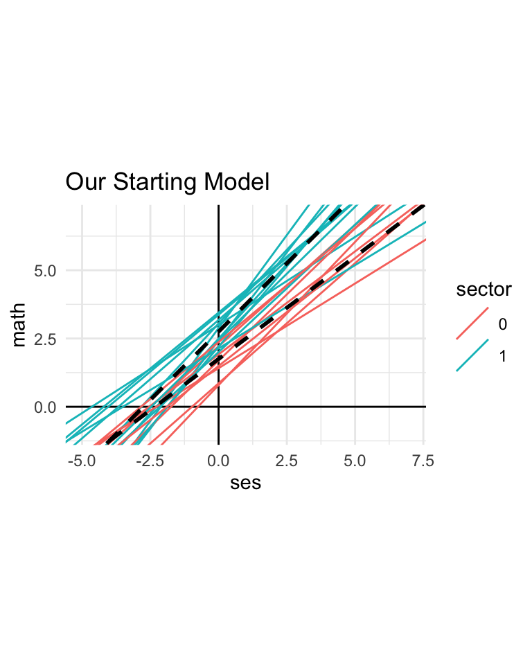
\[ \begin{pmatrix} u_{0j} \\ u_{1j} \end{pmatrix} \sim N \left( \begin{pmatrix} 0 \\ 0 \end{pmatrix}, \begin{pmatrix} 0.5^2 & 0 \\ & 0.2^2 \end{pmatrix} \right) \] For this model, with the parameters listed above, we get this:

Each line represents the regression line of math achievement on SES for that school (assuming we had infinite number of students in that school so we knew the line perfectly). The dashed lines show the overall public and Catholic regression lines. Our model says our schools are from two groups, and that the schools themselves vary by group (due to the random intercepts and slopes).

23.1 Null hypotheses on slopes

Now consider three different null hypothesis for the slope:

• \(\tau_{11} = 0\): This removes the random slope term. Note that this also implies \(\tau_{01}\) = 0.
• \(\gamma_{10} = 0\): This removes the overall average slope. We still allow individual schools to vary, and also for Catholic schools to be systematically different from public.
• \(\gamma_{11} = 0\): This removes systematic differences between Catholic and public schools.

We are going to generate data where everything is as the original model except for the null. We will then see how the data look different. Witness!

No random slope still gives different lines for each school, but they are very similar. First, our catholic schools all have one slope and the public schools another. The only difference is we allow the intercepts to vary, which gives the two bundles of lines.

No average slope means our public school slopes are 0, on average. Note the Catholic schools have a positive slope on average–this is due to the \(\gamma_{11}\) term.

Finally, if \(\gamma_{11} = 0\), then our Catholic and public slopes are all centered around the average slope of \(\gamma_{10}\)–but each school still has its own slope and the Catholic schools are still shifted higher

23.2 And what about intercepts?

Let’s do things to the school level intercepts:

• \(\tau_{00} = 0\): This removes the random intercept, but still lets the slopes vary. This is not something we would normally think would happen in practice, but it helps us see how the different parameters matter.
• \(\gamma_{01} = 0\): This means there is no shift in intercepts between Catholic and public schools.
• \(\gamma_{00} = 0\): This means that the public schools overall grand intercept is 0.

In all of the above, we are leaving the slope part of our model alone. Each school’s intercept is calculated from the grand intercept, the shift due to being Catholic, and the random intercept. Changing them changes things like this:

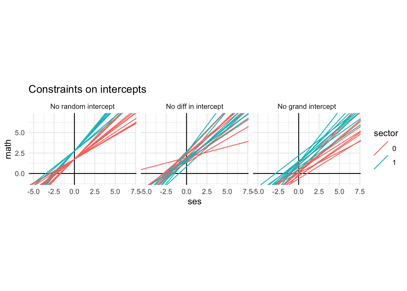
In the first plot, note how all the lines go through the same intercept point. The varying slopes give different lines.

The second plot has the Catholic and public schools sharing the same intercepts, but the Catholic schools have steeper slopes in general.

The third plot lowers the schools so the public school intercepts are 0 on average. The Catholic schools are still shifted higher by \(\gamma_{01}\).

23.3 And what are the taus?

Let’s drop all the Catholic and public differences (i.e., \(\gamma_{01} = \gamma_{11} = 0\)) and crank up the \(tau\) values:

• \(\tau_{00} = BIG\): The intercepts vary a lot.
• \(\tau_{11} = BIG\): The slopes vary a lot.
• \(\tau_{01} = BIG\): The covariance is large (i.e., the correlation of the random intercepts and slopes is very positive)

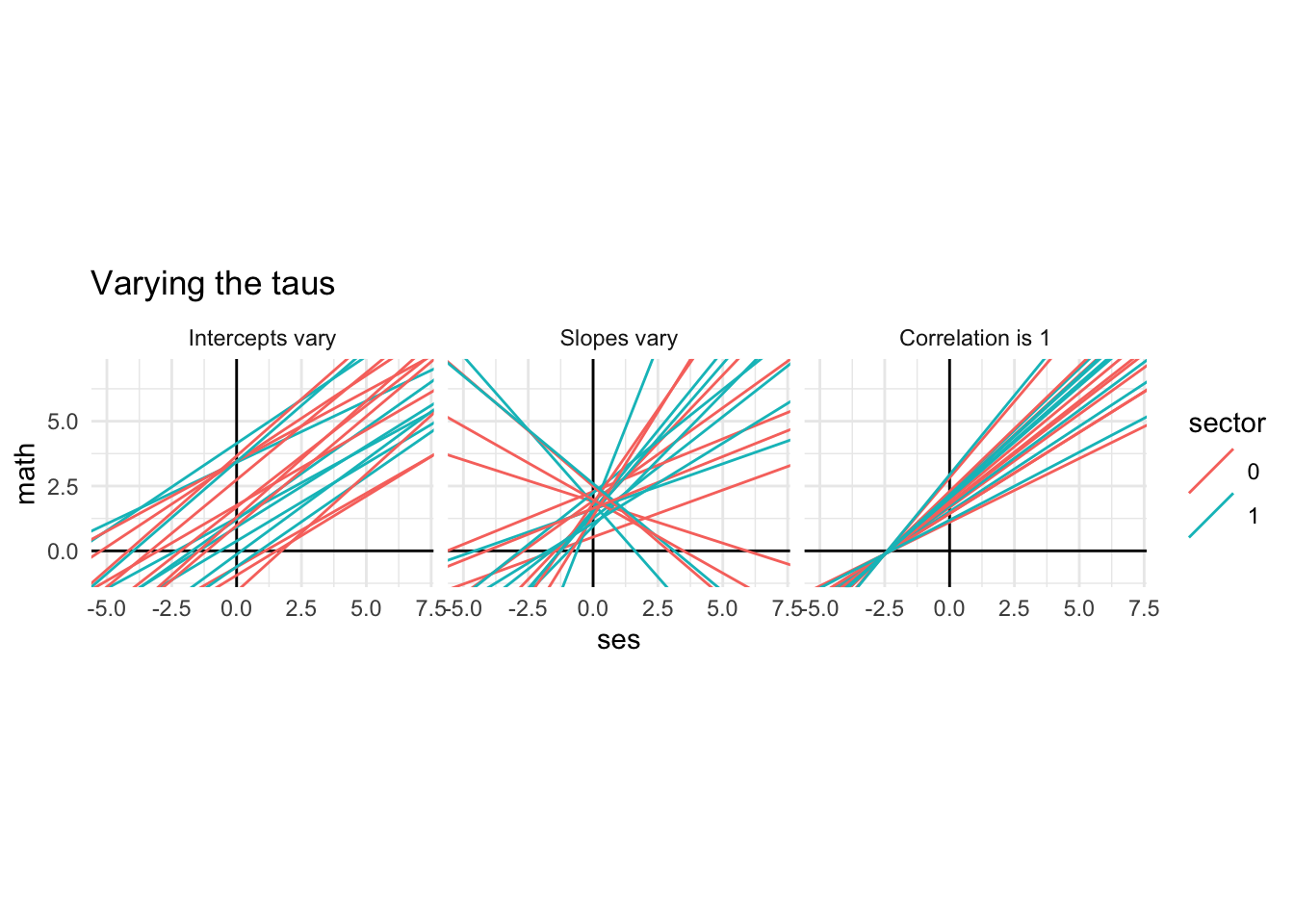
In the first plot, our lines are scattered vertically a lot, and in the second plot our slopes are all over the place. In the third plot, the steepest slope has the highest intercept.