In this chapter we outline a few simple checks you might conduct on a fitted random effects model to check for extreme outliers and whatnot.
first, let’s fit a random intercept model to our High School & Beyond data:
m1 <-lmer(mathach ~1+ ses + (1|schoolid), data=dat)arm::display(m1)
lmer(formula = mathach ~ 1 + ses + (1 | schoolid), data = dat)
            coef.est coef.se
(Intercept) 12.66     0.19
ses          2.39     0.11

Error terms:
 Groups   Name        Std.Dev.
 schoolid (Intercept) 2.18
 Residual             6.09
---
number of obs: 7185, groups: schoolid, 160
AIC = 46653.2, DIC = 46637
deviance = 46641.0
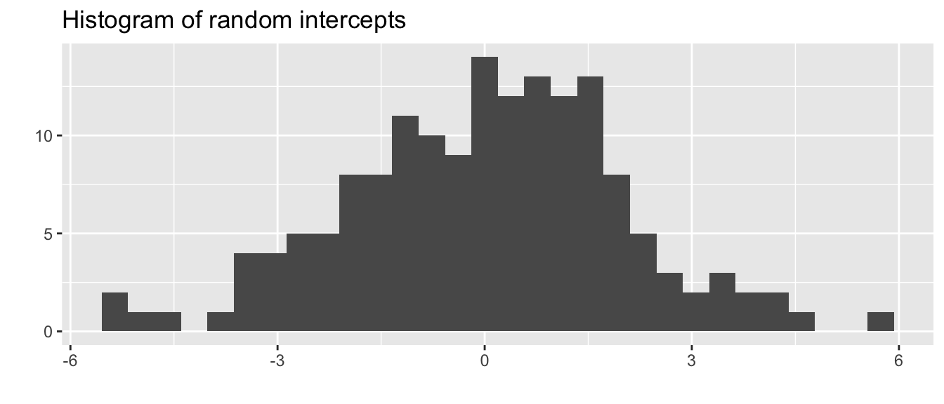
We can check if some of our assumptions are being grossly violated, i.e. residuals at all levels are normally distributed.
qplot(ranef(m1)$schoolid[,1],main ="Histogram of random intercepts", xlab="")
Warning: `qplot()` was deprecated in ggplot2 3.4.0.
`stat_bin()` using `bins = 30`. Pick better value `binwidth`.
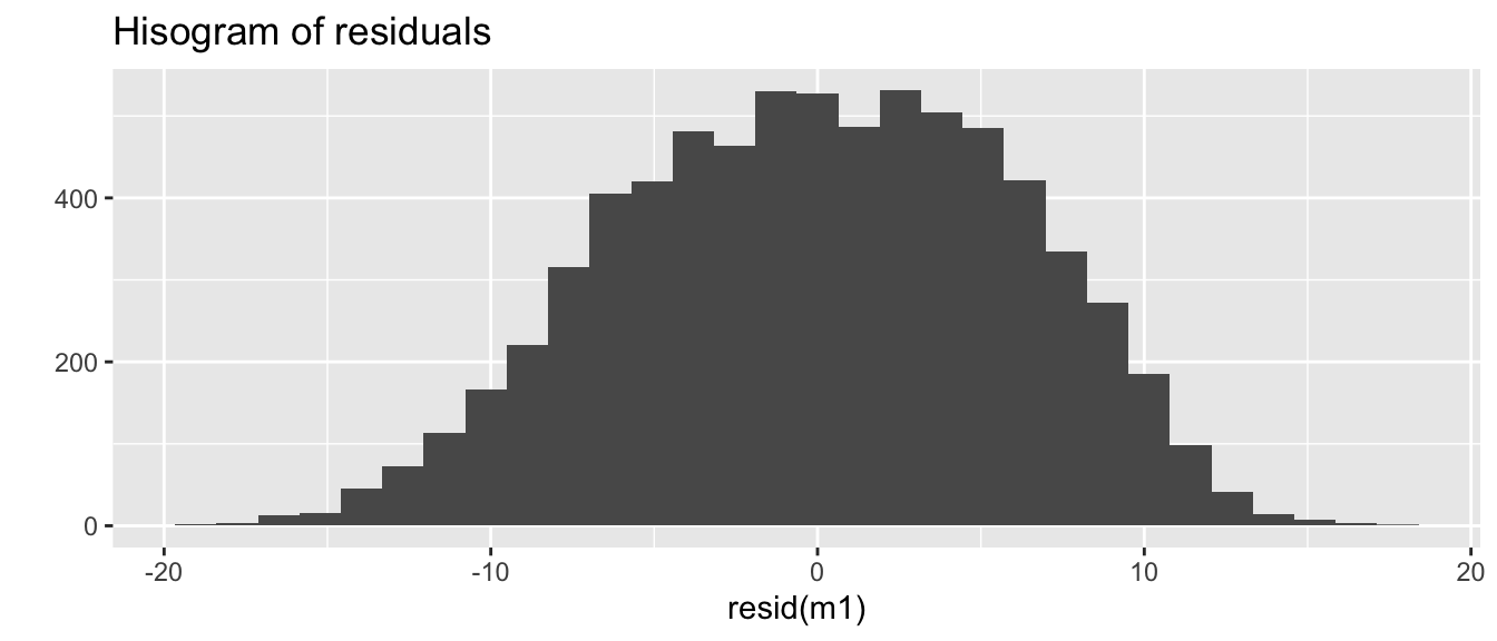
qplot(resid(m1), main ="Hisogram of residuals")
`stat_bin()` using `bins = 30`. Pick better value `binwidth`.
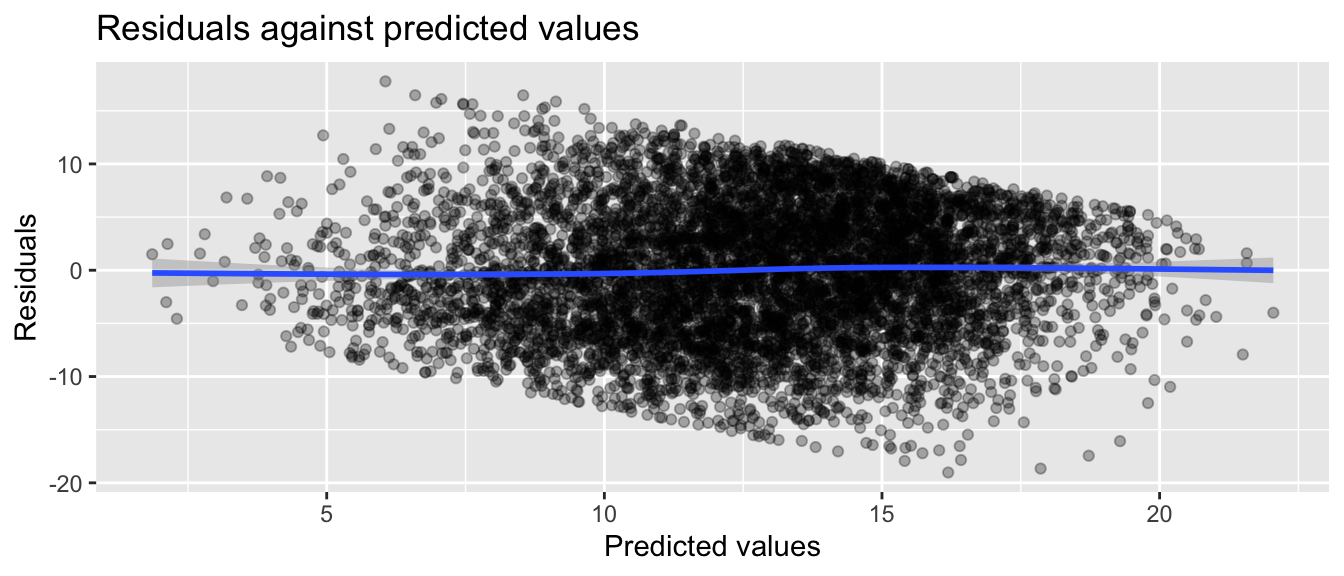
We can check for heteroskedasticity by plotting residuals against predicted values
dat$yhat =predict(m1) dat$resid =resid(m1)ggplot(dat, aes(yhat, resid)) +geom_point(alpha=0.3) +geom_smooth() +labs(title ="Residuals against predicted values",x ="Predicted values", y ="Residuals")
`geom_smooth()` using method = 'gam' and formula = 'y ~ s(x, bs = "cs")'
It looks reasonable (up to the discrete and bounded nature of our data). No major weird curves in the loess line through the residuals means linearity is a reasonable assumption. That being said, our nominal SEs around our loess line are tight, so the mild curve is probably evidence of some model misfit.
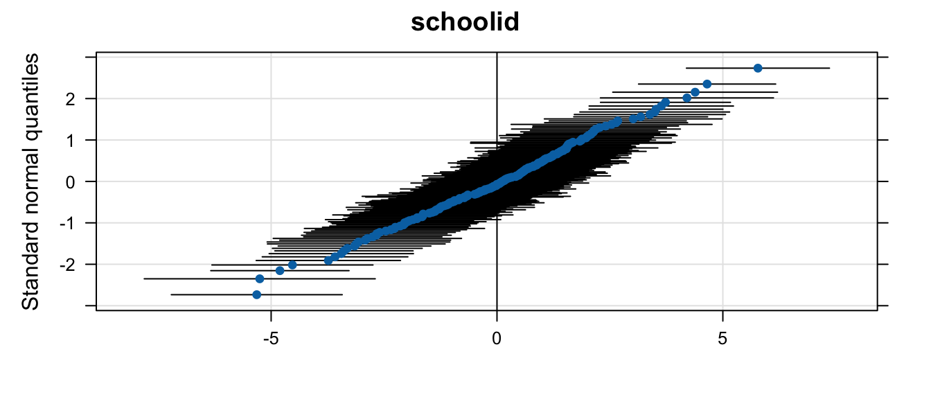
We can also look at the distribution of random effects using the lattice package