In this case study, we illustrate fitting a three level model (where we have time variation and then clusters) and then extracting the various components from it. This example is based on a dataset used in Rabe-Hesketh and Skrondal, chapter 8.10, but you don’t really need that text.
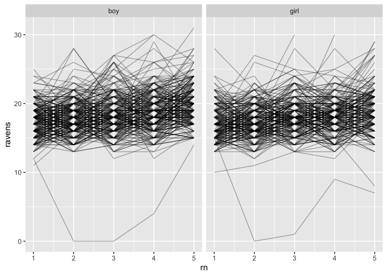
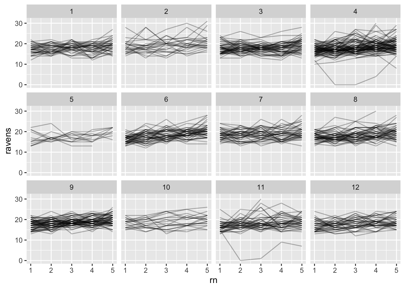
Shoving a lot of things under the rug, in this case study we have five measurements on a collection of kids in Kenya across time. We are interested in the impact of improved nutrition. The children are clustered in schools. This gives a three-level structure, and we are watching kids grow. The schools were treated with different nutrition programs.
43.1 Load the data
In the following we load the data and look at the first few lines. Lots of variables! The main ones are id (the identifier of the kid), treatment (the kind of treatment given to the school), schoolid (the identifier of the school), gender (the gender of the kid), and rn (the time variable). Our outcome is ravens (Raven’s colored progressive matrices assessment).
kenya =read.dta( "data/kenya.dta" )# look at first 9 variableshead( kenya[1:9], 3 )
Let’s fit a random slope model, letting kids grow over time.
Level 1: We have for individual \(i\) in school \(j\) at time \(t\): \[ Y_{ijt} = \beta_{0ij} + \beta_{1ij} (t-L) + \epsilon_{ijt} \]
Level 2: Each individual has their own growth curve. Their curve’s slope and intercepts varies around the school means: \[ \beta_{0ij} = \gamma_{00j} + \gamma_{01} gender_{ij} + u_{0ij} \]\[ \beta_{1ij} = \gamma_{10j} + \gamma_{11} gender_{ij} + u_{1ij} \] We also have that \((u_{0ij}, u_{1ij})\) are normally distributed with some 2x2 covariance matrix. We are forcing the impact of gender to be constant across schools, but are allowing girls and boys to grow at different rates. The average growth rate of a school can be different, as represented by the \(\gamma_{10j}\).
Level 3: Finally our school mean slope and intercepts are \[ \gamma_{0j} = \mu_{00} + w_{0i} \]\[ \gamma_{1j} = \mu_{10} + \mu_{11} meat_j + \mu_{12} milk_j + \mu_{13} calorie_j + w_{1i} \] For the rate of growth at a school we allow different slopes for different treatments (compared to baseline). The milk, meat, and calorie are the three different treatments applied. Due to random assignment, we do not expect treatment to be related to baseline outcome, so we do not have the treatment in the intercept term–this is rather unstandard and we would typically allow baseline differences to account for random imbalance in the treatment assignment. But we are following the textbook example here.
We also have that \((w_{0j}, w_{1j})\) are normally distributed with some 2x2 covariance matrix:
\(\mu_{00} = 17.41\) and \(\mu_{11} = 0.59\). The initial score for boys is 17.4, on average, with an average gain of 0.59 per year for control schools.
\(\gamma_{01} = -0.30\) and \(\gamma_{11} = -0.14\), giving estimates that girls score lower and gain slower than boys.
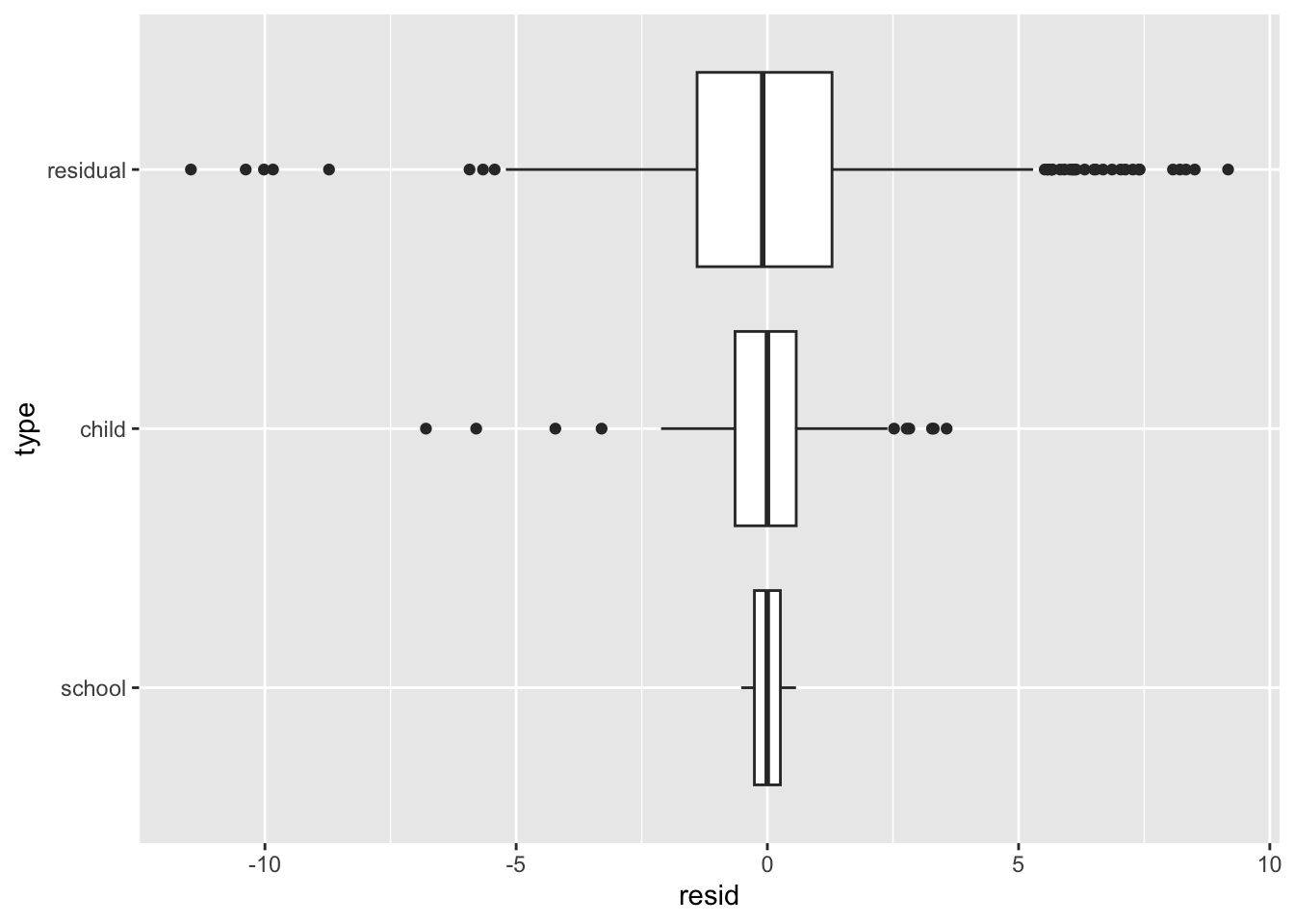
The school-level variation in initial expected Raven scores is 0.45 (this is the standard deviation of \(w_{0i}\)), relatively small compared to the individual variation of 1.40 (this is the standard deviation of \(u_{0ij}\)).
The correlation of the \(u_{0ij}\) and \(u_{1ij}\) is basically zero (estimated at -0.09).
The random effects for school has a covariance matrix \(\Sigma_{sch}\) of \[ \widehat{\Sigma}_{sch} = \left[
\begin{array}{cc}
0.45^2 & 0.45 \times 0.09 \times -0.99 \\
. & 0.09^2
\end{array}
\right] \] The very negative correlation suggests an extrapolation effect, and that perhaps we could drop the random slope for schools.
The treatment effects are estimated as \(\mu_{11}=0.17, \mu_{12}=-0.13\), and \(\mu_{13}=-0.02\).
P-values for these will not be small, however, as the standard errors are all 0.09.
We could try to look at uncertainty on our parameters using the confint( M1 ) command, but it turns out that it crashes for this model. This can happen, and our -0.99 correlation gives a hint as to why. Let’s first drop the random slope at the school level and then try:
We then have to puzzle out which confidence interval goes with what. The .sig01 is the variance of the kid (id:schoolid), which we can tell by the range it covers. Then the next must be correlation, and then the slope. This tells us we have no confidence the school random intercept is away from 0 (.sig04).
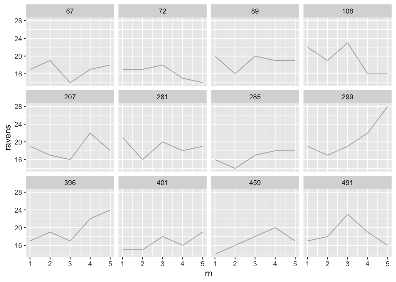
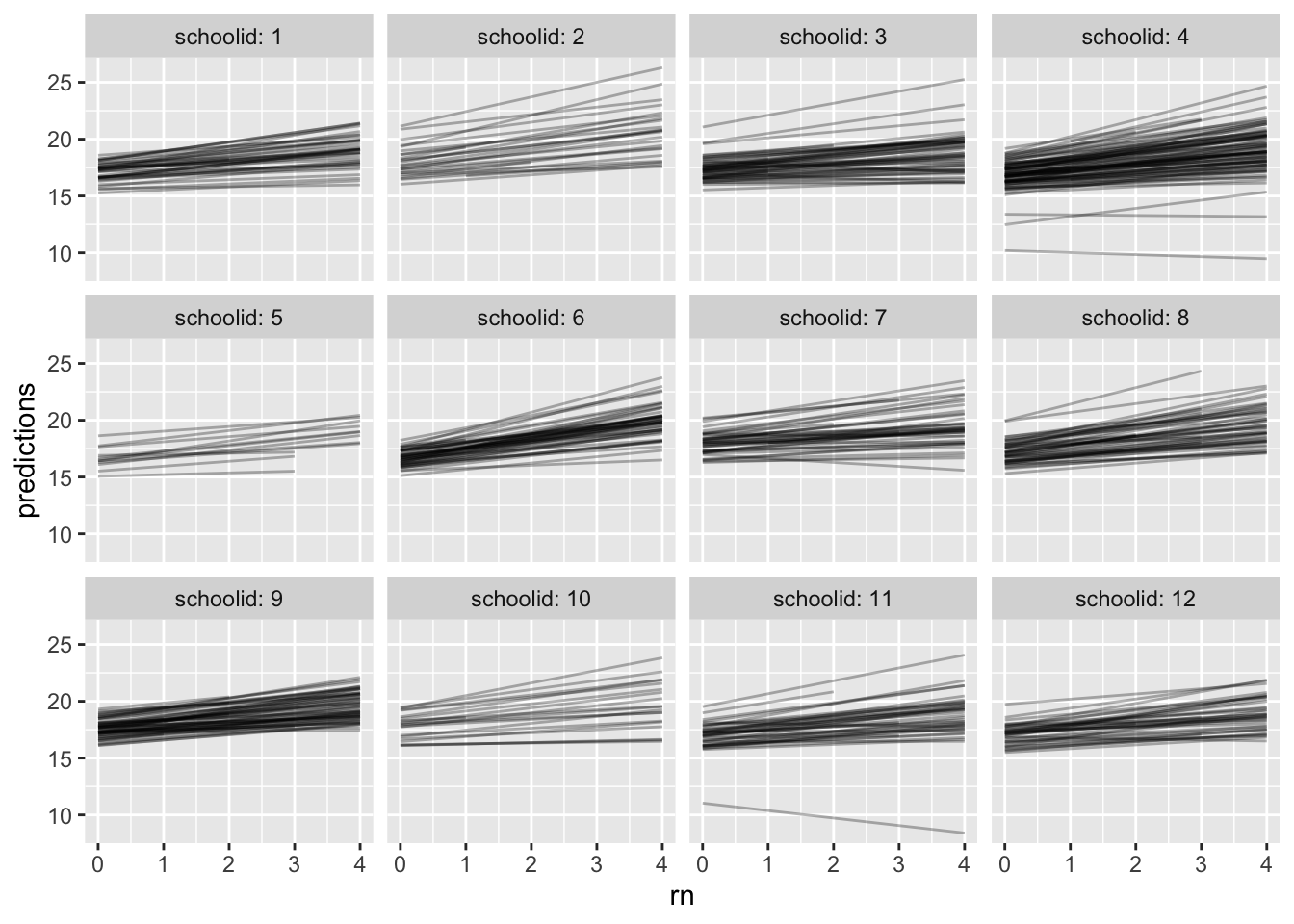
Generally individual curves are estimated to have positive slopes. The schools visually look quite similar; any school variation is small compared to individual variation.